Using Google Analytics with Sheets

If you didn’t already know, Google Sheets has a fantastic Google Analytics add-on that can be used to create custom reports in Google Sheets. For more information on the reporting capabilities of this tool, read this blog post from 2016, which will also teach you how to download the add-on and set up a custom report configuration. As an overview, this add-on allows you to:

• Quickly pull any data from Google Analytics (GA) accounts you have access to directly into a spreadsheet
• Easily compare historical data across custom time periods
• Filter and segment your data directly within Google Sheets
• Automate regular reporting
• Easily tweak your existing reports (which will be saved to Google Drive) to get new data

Beyond how to use the tool – we have free stuff!

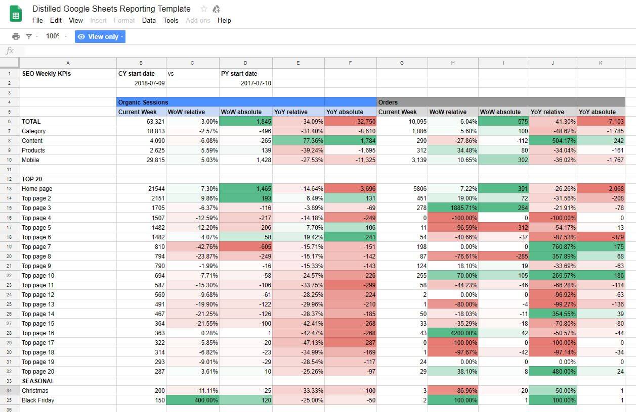
All the heaps of data you can pull with this tool are useful, but what if you want to quickly be able to compare data from your custom report configurations? Wouldn’t it be nice to have a reporting view that visually displays how your website is performing week-on-week (WoW) or year-on-year (YoY) by comparing the number of organic sessions and orders (and is near-automated)?

I thought so too.

Recently, I built a report using the Google Analytics add-on within Google Sheets. I have created a templated version of this report to share with you. Feel free to make a copy of it and use it as you please.

Here are some of the insights this report provides you with:

• Organic sessions and orders WoW and YoY for the entire website
• Organic sessions and orders WoW and YoY for different page types including category, content, product and seasonal pages
• Organic sessions and orders WoW and YoY for the homepage and a static top 20 pages
• Organic sessions and orders WoW and YoY for your mobile website

Using formulas, some regular expressions, and conditional formatting, their weekly SEO reporting process is now nearly automated using data from their Google Analytics.

Wait, can’t I do all of this in the GA interface already?

Not quite. Here are some of the benefits of this add-on over the standard GA interface:

• In the add-on, you can filter on dimensions or metrics that are not already included in your report. In the GA interface if you’re looking at a report with landing pages as the only dimension, you can’t use filters to filter to just organic traffic. With the add-on, you can
  • You can do this in GA using a segment rather than a filter, but segments are more prone to causing issues with sampling than filters
• Once you have loaded in your data with the add-on, you can manipulate it without having to continually export files
• You can do multiple comparisons with the add-on (which I do in this report), whereas in GA you can only do two, i.e. either year on year or week on week comparisons, not both simultaneously
• Using the add-on can provide you with a single source of truth, rather than having all the additional data offered by GA that you may not want to be diving into
• Using conditional formatting in Google Sheets means that I have been able to flag varying degrees of positive or negative changes by colour

How you can make this report your own

This blog post will walk you through why the report is useful, how you can customise it, and then if you’re curious, I’ve also gone into further detail in an appendix below how the report works. This will also be useful for any potential de-bugging you may have to do.

With the following instructions, even if you’re a beginner to things like regular expressions and Excel/Google Sheets formulas, you should still be able to customise the report and use it yourself.

To build the report I’ve used regular expressions within the reporting configuration to filter to specific page types that I wanted, and then in the “Comparisons” sheet, I’ve used formulas to pull the data from the sheets to then get WoW and YoY comparisons. All of this takes place within the sole Google Sheet.

For a one-time report, this would likely not be worth the time invested, but if you or a client have a need for standardised, ongoing reporting – and you have access to the GA data for the account – then this template can be a great way to give you quick, easy insight into your organic traffic trends.

It saves me close to an hour of time a week – or almost 6 working days a year.

What you will need to customise this report

To make this report your own, you’ll need:

• To download the Google Analytics add-on for Google Sheets (instructions are here)
• Access to the GA account you want to report on
• Your GA View ID (instructions on how to find this here)

Other resources you may find useful:

• GA’s Query Explorer – can be used to test the output of different combinations of metric and dimension filters
• GA Reporting API – lists and describes all the dimensions and metrics available through the Core Reporting API

Why this report is useful

This report uses conditional formatting to make any significant positive or negative changes stand out. It also uses both macro-scale views of the website trends and more detailed views. At the top, it has the total sessions and orders for the entire website, plus the WoW and YoY comparisons, and as you go further down the report it becomes more granular.

I built this report so I could get a better idea of how specific parts of a website were performing. The primary pages I have reported on are the category pages, content pages, product pages and mobile pages. Following that, I have put in the data for a list of the top 20 pages, including the home page. At the end, there is a section for seasonal pages.

The top 20 pages that it reports on are static. These were pre-determined by looking at those pages that consistently had the highest organic sessions. We opted to use a static top 20 rather than the actual top 20 by sessions per week because using the actual would require updating the SUMIF formulas each time the report was run.

This is a report that I update weekly. The date formulas are calculated based on whatever today’s date is and are then used in the report configuration.

This allows the dates to update on their own without me manually having to change them each time I want to run the report. I just had to then schedule the report to run weekly and BAM! – no hands necessary.

To set an auto-run for your report, go to Add-ons > Google Analytics > Schedule Reports, check “Enable reports to run automatically” and then set the time and frequency you want your report to run.

This has made my life much easier, and hopefully sharing it will make your life easier too.

How to customise this report

In this report you are going to have to customise:

• Your report configurations
• The dates you want this to run
• The primary page types you want to compare (we have category pages, content pages, product pages and mobile)
• The top 20 pages you wish to report on (you might choose not to use this)
• Your seasonal pages, if applicable

Necessary changes – Report Configurations

First level customisation

To learn how to set up and run report configurations, the blog post I referenced at the beginning can help you. For the purpose of this post, I’ll just focus on where you’ll need to tweak it for your website or client.

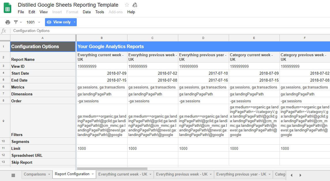
You will need to put in the View ID you want to report on (Row 3), and you will have to edit the regular expressions in the filters section (Row 9) to make them unique to your client, which I will cover below.

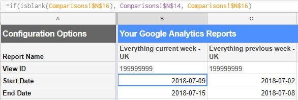
The dates I am using (Rows 4-5) are references to those I have in the comparisons tab. If you want to use different dates, you can either manually change them here, or in the next section, I explain how the date formulas work. Here’s a screenshot of the formula in cell B4 so you can see what I am talking about:

You also are likely going to want to change the Report Name (Row 2) for each column. If you do, be sure that you clearly label each section. The Report Name becomes the name of the sheet that is generated once you run the report, and later the name used in the formulas in the Comparisons tab.

Note that when you change the Report Name, it won’t replace the old one but will instead just create a new one. You’ll have to manually delete the old, unwanted sheets.

Updating the regular expressions

There are two parts of the regular expression that are unique to the website that you will have to update.

The first section that you’ll have to update is where I had to filter out PPC data that was being mistakenly reported as organic by GA.  For this site, PPC data could be identified with any URL that contained either “gclid”, “cm_mmc”, “newsl”, or “google” – this is likely to be different for you, so change what is in the quotations to reflect this.

This was being reported as organic because of the tagging used for PPC data was initially intended for a different reporting platform, so it may not be a problem for you. If so, you can delete this section.

If this is not a problem for you, then you can go ahead and delete this part of the Filters section (everything following ga:medium==organic in cells B9-D9 of the Report Configuration tab).

The second update you’ll have to make to the regular expressions are to those used in the Filter sections for all the columns aside from the ‘Everything’ ones (cells E9-P9). These are used to identify the part of the URL path you want to filter on.

Each filter is separated by a semi-colon, so if you want to add anything to these filters be sure to have that in there. Semi-colons mean “AND” in the Core Reporting API. For commas, you use “OR”.

Here is the ‘everything’ section:

ga:medium==organic;ga:landingPagePath!@gclid;ga:landingPagePath!@cm_mmc;ga:landingPagePath!@newsl;ga:landingPagePath!@google

Aside from ga:medium==organic (which just filters to organic sessions only) this just filters out PPC data.

I’ve copied this expression across all of my sections, but for the sections on specific page types I’ve also included another regular expression to get the specific URLs I am looking for, highlighted below.  For these sections, you’ll see variations of this:

ga:medium==organic;ga:landingPagePath=~\/category\/;ga:landingPagePath!@gclid;ga:landingPagePath!@cm_mmc;ga:landingPagePath!@newsl;ga:landingPagePath!@google

For this example, it was filtering for URLs containing “/category/”. This filters that report down to just our client’s category pages. Again, you can customise this regular expression to your unique website or client. Be sure to escape any slashes you use in this section with a backslash.

The mobile sections (cells N9-P9) were a bit different, as this is a defined dimension in GA. You’ll see in those columns that I just added in “ga:deviceCategory==mobile” after the filter for organic.

Once all that is done you can run your reports and move on to customising your Comparisons tab.

Necessary changes – Comparisons tab

Date formulas

The date formulas in cells M13:S18 further automate the reporting. The report defines a week as Monday to Sunday as this was how our client defined theirs, so if this is different for you, you’ll have to change it. If you’re curious how these specific formulas work, I have covered it in more detail in the appendix.

If you do change this section, make sure that the dates are formatted as YYYY-MM-DD. To do this, go to Format > Number > More formats > More date and time formats.

I’ve also left space to enter custom start and end dates. The specific client this was built for wanted to be able to compare odd weeks for their YoY comparisons around specific holidays. These dates will only be used if cells N16-S16 are not blank.

Google Sheets formulas – for primary, top 20 and seasonal pages

Once you’re happy with the dates, the primary thing you need to update are formulas, specifically the names of the sheets being referenced and the criteria that define the pages you want to report on.

If you are getting errors when you customise the formulas, especially #N/A! errors, try re-running the cells in the comparisons sheet first by just highlighting and pressing enter.

For the primary pages at the top in cells B6:K10, if you have changed the Report Names from the previous section you only have to update the sheet names being referenced. You’ll also have to do this for the following sections.

When you’re doing this, be sure not to mix up previous week and previous year.

This can be a long and irritating process. One thing I found that helped speed it up was another Google Sheets add-on Advanced Find and Replace. This lets you use the find and replace function within formulas, which means you can simply find “Everything current week – UK” and replace it with whatever alternative you have.

This plug in has a free trial, and once that is up you can only use it once a day – so make the most of it while you have it! If you know of any other free alternatives, I’d love to hear about them.

The formulas in the top 20 pages, cells B13:K24, have slightly different formulas are different depending on the page type.

Where I’ve highlighted in the formula below is the part of this formula you’ll have to change to match your specific page type. This is from cell B14:

=SUMIF(‘Everything current week – UK’!$A:$A,”*”&”/top page 2/“,’Everything current week – UK’!$B:$B)

The number you’re seeing is a sum of all the pages with /top page 2/ in the URL from the Results Breakdown in my Everything current week – UK tab, shown below.

For the seasonal section in cells B34:K35, you’ll just have to replace where I have either “christmas” or “black-friday” to include whatever specific seasonal term you want to report on. Remember, this must be a reference that is included in the URLs.

Other changes you can make – Report Configuration

For metrics, I have used sessions and transactions, but this can be adjusted if there is a different metric you wish to report on. Just be sure to change the headings in the comparison tab so you remember what you’re reporting on.

For dimensions, I have used the landing pages. Again, you can adjust this if you wish to, for example, report on keywords instead.

I’ve set the order to be in descending rather than ascending. This organises the data but also helped to determine the top 20 pages.

I have set the limits on these to 1,000. I did this because I only really cared about the specific data for the top pages. The limit does not change the total number that is reported, it just limits the number of rows.

Unfortunately, this is also where I have to talk about sampling. In my report tabs in cells A6 and B6 it says “Contains Sampled Data, No”. If your data is being highly sampled then you need to decide if that will be a roadblock for you or not.

Here is a resource with some ways to get around sampled data.

It’s reporting time

If you’ve made the above changes, once you run your reports with the updates to your Report Configuration, you should have a Google Sheet reporting on your specific data.

As promised, I’ve added an appendix to this post below for those of you that are curious to know in more detail how it works.

Happy reporting!

Appendix: How this report works, if you’re curious

Main report formulas

Totals, WoW and YoY for top report section

Columns B and G for the top section simply pull out whatever number is reported for the total sessions and total orders from each sheet. This is useful not only because it brings all the absolute numbers into one place, but also because I can now reference these cells in formulas.

For WoW relative (Column C), I’ve again referenced those same cells, but created a percentage with a (Current – Previous)/Previous formula.

Column D uses the percentages generated in Column C to extract the absolute number differences.

For YoY relative (Column E), I’ve followed the same exact method, just referencing the data for the previous year rather than the previous week. Again, I used these numbers to extract out the absolute numbers seen in Column F.

The grey orders section does the exact same thing, but instead references the cell in each respective configuration with the order total, rather than sessions.

I’ve also wrapped these formulas in IFERRORs, to prevent the sheet from having any error messages. This was primarily for aesthetics, although it is worth noting that sometimes this can lend to it saying there was a 0% change, when maybe there was a 100% increase as that page type did not exist in the previous year.

Date formulas

Our client wanted weekly reporting comparing weeks that run from Monday to Sunday as this was how our client defined theirs. Since GA weeks run from Sunday to Saturday, this had to be customised.

These dates are calculated based off the “=TODAY()” date in cell M14, as well as the first day of last year calculated in M16, the first Monday of last year in M18, and the week numbers in cells O12 and Q12.

Because these dates are calculated automatically here, in the Report Configuration tab I can simply reference the specific cells from my Comparisons sheet, rather than manually having to enter the dates each time I run the report. This also made it so I can set this report to run automatically every Monday morning before I get into the office.

You’ll also notice that below the dates I have left space to enter custom start and end dates, this is again because the specific client this was built for sometimes wants to compare odd weeks for their YoY comparisons to account for specific holidays.

In the Report Configuration sheet, I have an IF formula in the cells that says, if the custom cells are blank then use the usual date, if they are not, then use those. On those occasions, it does mean I have to manually run the reports, but I guess you can’t have everything.

Top 20-page reporting

The Top 20-page section is where the formulas get a bit beastly, but this was something the client specifically requested. We initially wanted it to report on the top 20 pages from each week, but that wasn’t possible using formulas, as we needed something static to reference.

For these, I used a SUMIF formula. For example, in cell C13 I have this formula to report the WoW relative number for the home page:

=IFERROR((SUMIF('Everything current week - UK'!A:A,"*"&".co.uk/",'Everything current week - UK'!B:B)-SUMIF('Everything previous week - UK'!A:A,"*"&".co.uk/",'Everything previous week - UK'!B:B))/SUMIF('Everything previous week - UK'!A:A,"*"&".co.uk/",'Everything previous week - UK'!B:B),0)

Again, the IFERROR statement wrapped around my formula is just to clean things up so lets drop that and break down what the rest of this formula is doing.

=(SUMIF('Everything current week - UK'!A:A,"*"&".co.uk/",'Everything current week - UK'!B:B)-SUMIF('Everything previous week - UK'!A:A,"*"&".co.uk/",'Everything previous week - UK'!B:B))/SUMIF('Everything previous week - UK'!A:A,"*"&".co.uk/",'Everything previous week - UK'!B:B)

The SUMIF formula sums up cells if they meet specific criteria. It works by defining the range, in this case ‘Everything current week – UK’!A:A (every row in column A of the sheet Everything current week – UK), and then the criteria that you want to be summed. Here, it is all cells which include anything and end with “.co.uk/”.

Lastly, you define the sum range, which is the range to be summed if it is different from the original range defined. We’ve used this here because we want the sum of all the sessions, not the landing page paths. That whole thing spits out the sum of all the sessions on the homepage for the current week. I’ve then subtracted from that number the sum of all the sessions for the previous week.

Finally, I’ve divided it by the sum of all the sessions of the previous week to get the percent change.I set formatting rules in these cells to format the numbers as a percentage, but you could also just add that the formula to multiply by 100. So within these cells there are two things you are going to have to customise (1) the names of the sheets being referenced, and (2) the criteria that define the pages that you want to report on. You’ll notice that in the top 20 pages, these are different depending on the page type (they have been intentionally changed for discretion).